Measuring Power and CdA

When you’re cycling your energy is spent either climbing hills or pushing air out of the way - those are the two main “sinks” of energy.

The first - climbing hills - is easy to calculate given elevation data. The second depends on your speed (squared), the cross-section area you present (A), and a constant (Cd). The area and constant together are known as CdA.

Here I measure CdA and use it, together with the elevation data, to estimate power output.

• Previous Work
• A Statistical Approach to CdA
  • Physics
  • Coasting
  • Calculating CdA and Crr
  • Data Exploration
  • Final Measurement
• Power Estimates
  • Calculation
  • Results
• Configuration
  • Theory
  • Practice
• Summary
• Update - Now with Crr

Previous Work

I’m not the first to have thought of this. This document describes an approach to measure both CdA and Crr (rolling resistance) by making test rides.

A Statistical Approach to CdA

However, I’m stuck at home injured, so I want to derive CdA from “normal” ride data I already have, without a power meter.

Physics

The physics is pretty simple. If we know the bike’s height and speed at two different points, and the distance between them, then:

• The total energy “added” to the system is the gravitational potential energy from a drop in height (going downhill) plus any extra work done pedaling.

• The total energy “removed” from the system is via aerodynamic drag plus braking plus rolling resistance.

• The difference between energy input and output will be seen as a difference in speed before and after (kinetic energy), ignoring losses due to braking.

That’s a fair number of variables, but we can simplify things by:

• Only using data where the ride is not pedaling (where cadence is low).

• Assuming that there is no wind (which would affect aerodynamic drag).

• Ignoring rolling resistance (which should be relatively small).

• Treating the braking as “noise”. This will become clearer later, but basically we can hope that braking will be seen as erroneous measurements that give high CdA values.

Another way of saying this is that we will divide the ride into many small sections. In some the rider will be braking, and those will give bad results. But hopefully there are enough sections without braking that we can see some kind of consensus emerge.

Coasting

First, we need to find sections of the ride where the rider is not pedaling. For this we need the cadence sensor.

The SQL query here is intimidating, but not as complex as it looks. It is trying to find start and finish points (s and f) where:

• The cadence is less than max_cadence at those points and at all points between.

• Outside the two points (at ss and ff) the cadence is more than max_cadence (so we have the largest section possible).

• All points are in the same “timespan” (lap / autopause block).

• The average speed across the whole segment is at least min_speed.

• The total time across the whole segment is at least min_time.

Segments found are added to the ActivityBookmark table.

Calculating CdA and Crr

Once we have found the segments we can look at each “step” (recording interval) in the segment. At the start and end of each step we know the location, distance and speed (v), so we can calculate:

• Elevation change, h.

• The distance traveled, d.

• The gravitational potential energy gained (or lost, if climbing). This is m x g x h where m is mass (rider and bike) and g is gravitational acceleration (9.8 m/s).

• The kinetic energy before and after (1/2 x m x v^2).

• The average of the squared speed avg_v2, assuming that speed varies linearly (constant acceleration). You need to do a little calculus for this, but it turns out that it’s v_a^2 + v_a x v_b + v_b^2 where v_a is the speed at the start and v_b the speed at the end.

• The loss in energy due to air (CdA x p x avg_v2 x d) where p is air density (1.225kh/m^3).

• The loss in energy due to friction (Crr x d).

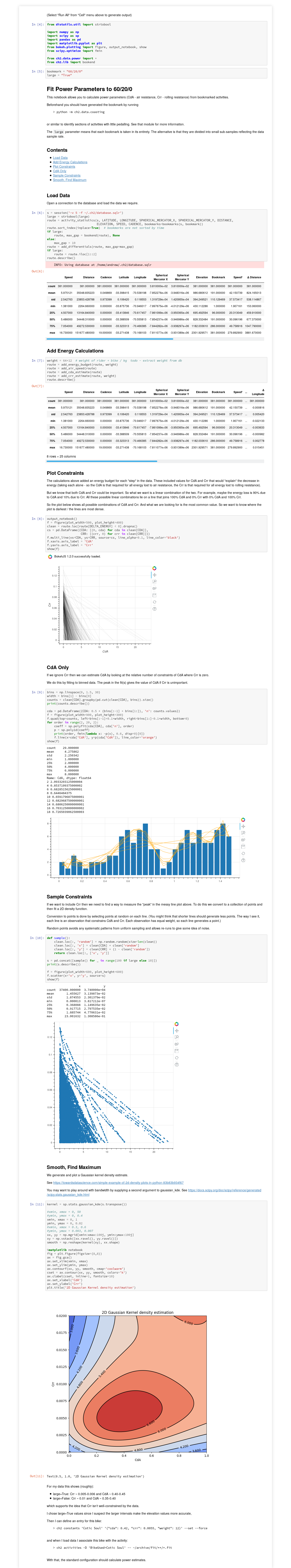
Data Exploration

From the energy balance described above we know that the change in energy can be attributed to resistance from air plus friction. If we don’t know CdA or Crr then all we have is their sum. This means that, for each step we can plot a line on the graph of CdA n Crr (the line shows all points that sum to give the same energy loss).

That plot looks like this:

Zoomed in on the x-axis (CdA) we can see:

There’s clearly a peak around a value of CdA at something like 0.5. But there’s no evidence of any kind of preferred value in the y direction.

I was hoping (optimistically) that we would see a preference for a certain value of Crr (ie more lines crossing at a certain y value) because the different dependency on speed for the two coefficients means that they should be distinguisable in observations made at different speeds. But I think here we’re just getting too much noise from braking (which we can’t control for, and which appears as rolling resistance).

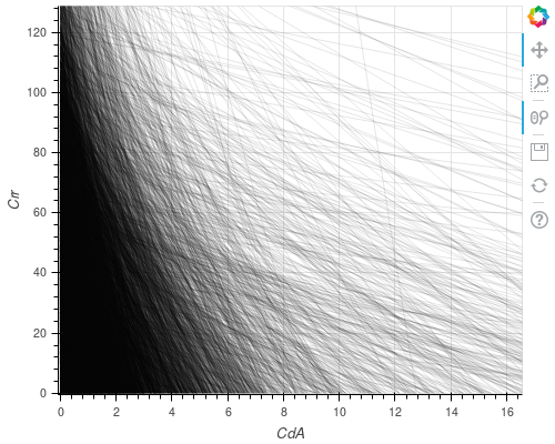
Final Measurement

Given the above, we’ll assume Crr is zero and calculate CdA alone. This is equivalent to counting the number of lines that cross the x axis in the plot above. Viewed as a histogram:

The curves are polynomials fit to the data - a way of smoothing the data to find the maximum. From those, the maximum is somewhere around 0.44.

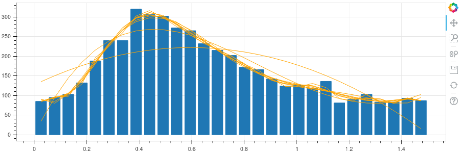
Power Estimates

Calculation

Given an estimate of CdA it’s then possible, for any segment of a route, to calculate the overall energy balance. If we continue to ignore braking then the sum of any (1) energy gained (indicated by increased speed or height) and (2) energy lost (via CdA) must be equal, numerically, to the average power multiplied by the time interval.

This logic can be seen in the code here. In particular,

df[POWER] = (df[DELTA_ENERGY] + df[LOSS]) / df[DELTA_TIME]

Results

The plot above shows a typical example taken from an activity report. Values are calculated using the “natural” sampling of the GPS file - the energy balance is calculated at each GPS position. The results are very noisy (even when, as here, median smoothed over 60s), but have fairly reasonable values.

Limitations include:

• Braking is ignored and effectively “uses up” some power, leading to under-estimates.

• I suspect elevation is over-smoothed, but I am unsure how this would affect estimates.

• “Negative” power is simply ignored (after smoothing).

• Wind speed and direction is ignored.

• Crr is ignored (and could be significant for MTB on rough ground).

• I have no measured power data to calibrate.

• The current implementation uses “constant” parameters for mass, etc. Some of these could be taken from the database itself.

Configuration

Theory

Configuring the power calculation is complex because the calculations cross-reference values from elsewhere in the database.

By default the pipeline is configured as:

> sqlite3 ~/.ch2/database-version.sql "select * from pipeline where cls like '%Power%'"
3|0|ch2.stats.calculate.power.ExtendedPowerCalculator|[]|{"owner_in": "[unused - data via activity_statistics]", "power": "PowerEstimate.Bike"}|20

which shows that the power variable references the constant PowerEstimate.Bike:

> ch2 constants show PowerEstimate.Bike
PowerEstimate.Bike: Data needed to estimate power - see Power reftuple
1970-01-01 00:00:00+00:00: {"bike": "${Constant:Power.${SegmentReader:kit}:None}", "rider_weight": "${Topic:Weight:Topic \"Diary\" (d)}", "vary": ""}

That rather opaque expression contains the basic data used to calculate power.

Two entries are particularly important here:

• "rider_weight": "${Topic:Weight:Topic \"Diary\" (d)}" - this sets rider_weight to be the most recent value of the Weight statistic from the diary.

• "bike": "${Constant:Power.${SegmentReader:kit}:\ None}" - this sets bike to the value of a constant whose name depends on the kit specified when they data were loaded (see Tracking Equipment). For example

  > ch2 activities -D 'kit=cotic' ...
  

  In this case the constant used would be called Power.cotic which is defined as

  > ch2 constants show Power.cotic
  Power.cotic: Bike namedtuple values to calculate power for this kit
  1970-01-01 00:00:00+00:00: {"cda": 0.42, "crr": 0.0055, "weight": 12}
  

  and describes the parrameters for that particular bike.

Practice

• The pipeline is configured as part of the default configuration.

• The Weight variable in the diary is also part of the default configuration.

• The PowerEstimate.Bike constant is also part of the default configuration.

• The kit statistic should be set during activities import.

• The Power.cotic (or whatever name you use for your bike) constant must be added by the user:

  > ch2 constants add --single Power.cotic \
    --description 'Bike namedtuple values to calculate power for this kit' \
    --validate ch2.stats.calculate.power.Bike
  > ch2 constants set Power.cotic '{"cda": 0.42, "crr": 0.0055, "weight": 12}'
  

Summary

The data suggest that my CdA is around 0.44, which appears to be roughly correct. With this I can estimate power output. Again, the values are ballpark correct.

The code to generate bookmarks is here and can be run via:

> python -m ch2.uranus.coasting

Update - Now with Crr

[July 2019] - I have extended the notebook I used for the work above and added it as a template. If you run:

> ch2 jupyter show fit_power_parameters 'bookmark' True

the Jupyter page should be displayed. This now fits both CdA and Crr (despite what I said above!). For full details (including an explanation of the ‘bookmark’), see the template.

Below is a snaphshot of the template with my data: