2018-12-16

Nearby Activities

We all have favorite routes when cycling. But even when we repeat a ride we make small changes - ride a little further, take a short-cut home, explore a new diversion.

This is how Choochoo identifies these related routes.

Contents

• Design
  • Data Model
  • Algorithm
    • Measure Similarities
    • Cluster Activities
  • Configuration
    • Pipeline
    • Constants
• Results
  • Image
  • Diary
• Appendix - DIY

Design

Data Model

Two new tables are added to the database:

• ActivitySimilarity is the (half-)matrix of similarity measurements. For each pair of ActivityJournal IDs, it contains a float value, similarity, which is a measure of how similar the two routes were.

• ActivityNearby associates similar ActivityJournals into groups.

Algorithm

Nearby activities are grouped in two stages:

1. Similarities between pairs of activities are measured.
2. Using the measured similarity, activities are grouped into clusters.

Measure Similarities

This step compares each pair of activities. An activity can contain tens of thousands of GPS measurements.

The solution here:

• Is O(n log(n)). It is faster than quadratic, even though all pairs are considered.
• Is “weakly” incremental. It is less expensive to add a new activity than it is to re-process all activities, but the speed increase is only a constant factor.
• Is robust. The results are not strongly influenced by noise in the data or processing order.

In broad outline:

• Store points from previous activities in an RTree.

• For each point in a new activity:
  • Count the number of “nearby” points from other activities by querying the RTree,
  • Add the new points to the RTree.
• The similarity measure for any pair of activities is the ratio of the number of nearby points divided by the total number of points in the two datasets.

Nearby points are found by extending the Minimum Bounding Rectangle (MBR) around each point by a fixed amount (default 3m) and then checking for MBR overlap.

The RTree returns both the matched MBR and the ActivityJournal ID associated with the point. The MBR is stored so that multiple matches are counted just once.

No account is taken of ride direction. Segments of travel that are ridden in both directions will “score double.”

For incremental processing, points from previous activities must be stored in the tree, but querying can be skipped.

The crude metric used (tangential plane to a sphere) means that all calculations must be within a “small” area of latitude and longitude. In practice this is sufficiently large for rides that start from a single (eg home) location. It is also possible to configure and process multiple regions.

The similarity measure is symmetric and stored as a triangular matrix in ActivitySimilarity.

Cluster Activities

The data are clustered using DBSCAN with a minimum cluster size of 3. This is much faster than measuring similarities and is re-run completely when needed.

The distance metric is calculated from the similarity by subtracting the similarity from its maximum value and normalizing to 0-1.

The critical distance used to define clusters (“epsilon” in the DBSCAN algorithm) is chosen to maximize the number of clusters. The value is found using an adaptive grid search.

Configuration

Pipeline

Data are processed in Choochoo using an extensible pipeline of tasks. This work adds a new pipeline class, NearbyStatistics.

The default configuration includes one instance of this class, with parameters appropriate for Santiago, Chile (where I live). The next section describes how to modify these parameters.

To add further classes (for example, to add additional groups in separate locations), add further instances to the pipeline table in the database. This is best done using the add_nearby helper function in ch2.config.database.

Constants

The pipeline task reads parameters from a JSON encoded “constant” that can be modified by the user. In the default configuration this is called Nearby.Bike.

The current value can be displayed with:

> ch2 constants show Nearby.Bike
Nearby.Bike: Data needed to calculate nearby activities - see Nearby enum
1970-01-01 00:00:00+00:00: {"constraint": "Santiago.Bike", "activity_group": "Bike", "border": 3, "start": "1970", "finish": "2999", "latitude": -33.4, "longitude": -70.4, "height": 10, "width": 10}

A new value can be given using --set --force (force is needed because you are overwriting an existing value). For example:

> ch2 constants set --force Nearby.Bike '{"constraint": "London.Bike", "activity_group": "Bike", "border": 3, "start": "1970", "finish": "2999", "latitude": 51.5, "longitude": 0.1, "height": 10, "width": 10}'
INFO: Using database at /home/andrew/.ch2/database.sqln
INFO: Checking any previous values
INFO: Need to delete 1 ConstantJournal entries
INFO: Added value {"constraint": "London.Bike", "activity_group": "Bike", "border": 3, "start": "1970", "finish": "2999", "latitude": 51.5, "longitude": 0.1, "height": 10, "width": 10} at None for Nearby.Bike
WARNING: You may want to (re-)calculate statistics

Results

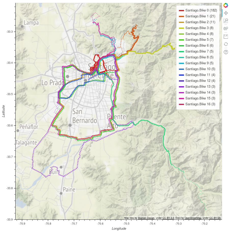
Image

The image above is generated in Jupyter using the nearby_activities template:

> ch2 jupyter show nearby_activities Santiago,Bike

In general the grouping makes intuitive sense.

Diary

Choochoo’s diary displays both “closest” matches and “most recent” matches, based on the similarity data. The grouping is not used here. Instead, similarity measures with a cut-off provides a more flexible set of references.

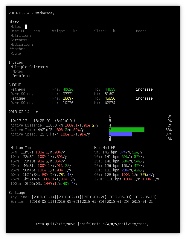
See the near-last lines, under “Santiago”. These are “links” that display the appropriate diary page when selected.

Appendix - DIY

To generate similar plots for your own rides:

• You need FIT data from your rides. If you use an online service for tracking exercise you can probably download these. For example, for Garmin, go here.

• Install Choochoo (the default config is sufficient).

• Adjust the configuration.

• Load your FIT data:

  > ch2 activities path/to/*.fit
  

• Start Jupyter:

  > ch2 jupyter show nearby_activities 
  

  which will automatically appear in your web browser.

• Open, modify and run notebooks/plot-group.ipynb. This has detailed configuration for my own data, but you can edit the script to tailor it to your own needs.

• You don’t need to use the nearby activities, of course. You can plot a single activity directly. Simply find the ActivityJournal ID, then load and plot the appropriate waypoints. Have fun.